Dimensionality Reduction for scATAC Data

There have been many different efforts to improve dimensionality reduction methods for scATAC-seq data, particularly considering that it is a relatively underexplored datatype when compared to scRNA-seq. With many different options, it can be somewhat confusing to follow the differences and pros/cons behind each method. The purpose of this post is to:

1. Highlight the major classes of methods that exist currently
2. Point out a very simple modification of LSI/LSA that we find works much better than the version of LSI/LSA many groups may be using
3. Show performance of selected methods on real-world data
4. Discuss the tradeoffs between sample-specific features and sample-agnostic features

I also provide an R markdown file that demonstrates how to use some of the methods here and reproduces all the analyses (including data downloads), which I hope is useful for exploring the methods discussed in this post.

R Markdown (HTML)

Many of the methods discussed here could, in principle, be applied to data from other single-cell epigenetic technologies, not just scATAC-seq.

Review of existing methods

At least in my view, there are two main classes of methods that exist currently, although each class is made up of several different potential approaches: methods that use metafeatures and methods that use genomic features.

Dimensionality through scoring of metafeatures

The idea employed by methods in this first category is that you can choose a set of metafeatures such as total overlap with existing peak sets (say different ChIP peaks), k-mers, motif hits, etc. and use a normalized/scaled version of the feature by cell count matrix as a reduced dimension representation of the dataset. This representation can then be used as input to t-SNE/UMAP, clustering methods, etc. In some of these cases, the feature by cell matrix can also be used to compute enrichments of motifs, which can be useful independent of dimensionality reduction.

I believe the first method developed that fell into this category was chromVar. Other methods that fall into this category include BROCKMAN and SCRAT. Lareau, Duarte, and Chew, et al. also recently applied similar methods in their study (k-mer count deviations).

Dimensionality reduction via genomic features

There have also been a number of approaches based on different types of genomic features. One of the initial challenges with scATAC-seq data was that the choice of features was not nearly as obvious as the choice in scRNA-seq data (genes). Much of the useful information contained in scATAC-seq data isn’t overlapping genes or easy to meaningfully associate with specific genes. In our experience, using gene-level scores as features in dimensionality reduction tends to result in substantial loss of resolution. We have tried gene body coverage, sums around genes (with or without peaks to constrain and with or without an exponential decay with distance), and methods that weight peaks according to their partial correlation with promoters (a version of activity scores as described in Cusanovich and Hill, et al. (Cell 2018)).

A number of different types of features have been by used by us and others with much more success than gene-level scores (at least in our hands):

1. Coverage within windows of the genome (generally 5kb in width)
2. Coverage within peaks (either derived from bulk data or merged peaks from across clustered subsets of the data)
3. Extended fragment overlaps used directly as a means for arriving at a distance metric (more on this later)

1 and 2 leave you with what is effectively a binary (due to sparse sampling of the genome) window/peak by cell matrix. You can then either transform this matrix in some way or directly calculate a distance matrix prior to doing a first round of linear dimensionality reduction, usually PCA via a fast matrix factorization approach like those implemented in IRLBA, which can then be used as input to clustering/further dimensionality reduction, etc. However, there are several ways that different groups have gone about this, all of which are geared towards the binary nature of the data.

In 3, no windows are used explicitly, rather, fragments are extended to a given length and then overlaps of fragments between cells are used to calculate distance metrics directly for input into dimensionality reduction. One could argue that this is technically not based on “features”, but I personally think it is ultimately similar enough to some of the other methods in this category that I have included it here.

Next, I will describe a few of the specific methods above in more detail.

LSI/LSA

LSI/LSA or Latent Semantic Indexing/Analysis (two existing terms used to refer to the same techique) is a very simple approach borrowed from topic modeling. You start with a binarized window or peak by cell matrix, and then perform a transformation called term-frequency inverse-document-frequency (TF-IDF) to provide some depth normalization and up-weight windows/peaks that appear less frequently in the population (the reasoning being that these are more likely to be informative). This has the added benefit of making the matrix non-binary. Generally, you would impose some minimum threshold for the rate of detection of a window/peak in a population to avoid amplifying noise. This transformed matrix can then be fed directly into PCA.

As I will discuss later, there are several different and valid ways out there to perform TF-IDF and the particular choice of method can have a substantial impact on performance, particularly for sparser datasets.

To my knowledge, Cusanovich, et al. (Science 2015) was the first study to use LSI/LSA on scATAC data (although the technique has been established for quite some time and applied in many other fields). Several other papers have used LSI/LSA such as Cusanovich, Reddington, and Garfield, et al. (Nature 2018), Cusanovich and Hill, et al. (Cell 2018), Chen, et al. (Nature Communications 2018), Satpathy and Granga, et al. (bioRxiv 2019), and the 10X genomics cellranger ATAC pipeline (implements both LSI/LSA and PLSI/PLSA). Note that this list may not be comprehensive.

Since LSI/LSA can be used on either windows or peaks, the specific uses in the literature mentioned above may vary with respect this choice (we have used both windows and peaks ourselves in different contexts for past publications).

PLSI/PLSA and LDA

Latent Dirichlet Allocation (LDA) and probabilistic LSI/LSA (PLSI/PLSA) are two other approaches borrowed from topic modeling. These techniques assume that there exist some underlying number of topics (if you were looking at documents, these might ultimately be interpretable as topics like politics, technology, etc., but in our case these might represent sets of windows/sites that share similar accessibility patterns and perhaps could be functionally related in some way) and that each observation (documents, or cells in our case) belongs to each topic with a given weight/probability. The goal is then to establish a probabilistic model that can help us find the underlying topics and assign each cell a probability of belonging to each of those topics.

PLSI is a probabilitic version of LSI that can be solved using either an expectation maximization (EM) approach or a non-negative matrix factorization (NNMF) approach. Rather than doing TF-IDF followed by PCA, EM or NNMF are used to find matrices that correspond to P(topic | document) and P(word | topic) (or P(topic | cell) and P(window/peak | topic) in the context of scATAC-seq data) distributions. You would pick the number of topics much like one would pick a number of principal components. More details can be found in a number of places, including towards data science. One of the potential benefits of PLSI/PLSA is that both matrices are very readily interpretable as probabilities, which is not quite so much the case in LSI/LSA (although the loadings from PCA can used to aid in interpretation).

LDA has a very similar goal to PLSI, but rather than using EM or NNMF, it places a Dirichlet priors over the P(topic | document) and P(word | topic) distributions and uses a Bayesian approach (usually some variant of Gibbs sampling) to solve the problem.

In the end, the P(topic | cell) matrix is a cell by topic matrix of probabilities which can then be used as a reduced dimension space. In practice this can then be used as something equivalent to the PCA space obtained from LSI/LSA. PLSI/PLSA and LDA are each much slower than LSI/LSA (LDA more so than PLSI), but are generally thought to be more accurate.

LDA is used in a tool called cisTopic described in González-Blas, Minnoye, et al. (Nature Methods 2019). PLSI/PLSA is available via the cellranger-atac pipeline as mentioned above, although I have not used it myself.

In our experience, LDA is slow enough that one would likely only want to apply it to peaks in practice (since they are often less numerous), although in principle one could apply LDA to a window by cell matrix.

Jaccard distances

Another alternative to LSI/LSA and LDA is to compute the Jaccard index (a metric meant for binary data) as a measure of similarity and use the resulting pairwise distance matrix as input into PCA (this would be, I believe, equivalent to classical multi-dimensional scaling although typically this would use a euclidean distance matrix). There are two main flavors of Jaccard-based approaches with which I am familiar:

1. Compute pairwise Jaccard index (similarity) based on window by cell matrix, performing post-hoc normalization to account for this metric being highly sensitive to differences in total reads per cell.
2. Extending all fragments to a larger length (say 1kb) and computing Jaccard indices directly based on extended fragment overlaps. Post-hoc normalization could be performed or cells could be downsampled to equal depth beforehand.

1 has been implemented in a recent pair of tools called SnapATAC/SnapTools, described in Fang, et al. (bioRxiv 2019). I’ll also comment on SnapTools/SnapATAC more later, as they are really nice tools more generally! In this instance the authors use the normalized pairwise Jaccard index matrix as input to PCA. Bing Ren’s group has also used earlier versions of this type of method in previous work like Preissl et al. (Nature Neuroscience 2018)

2 was described in Graybuck, et al. (bioRxiv 2019) and the authors downsample cells to 10,000 fragments each rather than performing normalization before using this matrix as input to t-SNE directly.

Other approaches based on genomic features

I found at least one other approach described in Lake, Chen, Sos, and Fan, et al. (Nature Biotechnology 2018), that models scATAC-seq data as a right-censored Poisson process (to account for the the binary nature of the data), and then uses the censored Poisson deviance residual matrix as input to PCA.

There are likely other approaches out there that I’m not aware of or that have not been published yet. You could imagine approaches like scVI, as described in Lopez et al. (Nature Methods 2018) or any one of several other autoencoder-based approaches being applied to scATAC-seq data with appropriate modifications to account for the fact that the underlying data would not follow a negative binomial distribution.

Important details when employing LSI/LSA

At this point, it is worth mentioning that since our group has used LSI/LSA extensively in the past, you should take my opinion here with a large grain of salt. For the comparisons below, I’ve done my best to try out other methods and use more than one dataset to give a relatively unbiased view.

Since our last publication using scATAC-seq data (Cusanovich and Hill, et al. [Cell 2018]), I had explored using cisTopic and found that it tended to work quite a bit better than our usual LSI/LSA method in many but not all cases.

We went on to notice even more substantial differences in sparser datasets and we were always a bit confused as to why LSI/LSA seemed to perform so poorly on very sparse datasets. After some digging, we arrived at the conclusion that much of the difference might be attributable to the way in which we and many (but not all) others have typically computed the TF matrix in the TF-IDF step of LSI/LSA rather than the difference in the matrix factorization procedures used in LSI/LSA and LDA.

Generally we (and many others) compute the TF matrix as (in R):

tf = t(t(count_matrix) / Matrix::colSums(count_matrix))

We would then compute the TF-IDF matrix using:

idf = log(1 + ncol(count_matrix) / Matrix::rowSums(count_matrix))
tfidf = tf * idf

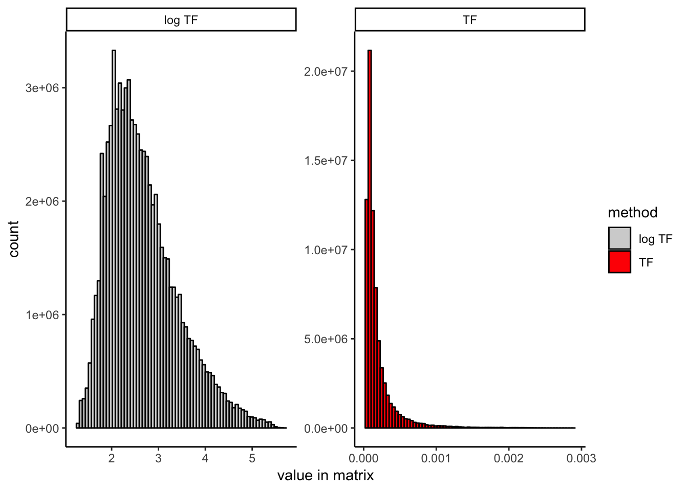
It turns out that in many scATAC-seq datasets (particularly if you are not pretty restrictive about which cells and sites you use as input as we have typically been in our papers), the tf term as calculated above will end up having strong outliers due to the distribution of total sites in cells.

Since the resulting TF-IDF transformed matrix is being used as input into SVD/PCA without any further normalization or scaling, if you do have strong outliers in the TF matrix, it is entirely expected that a method like PCA would tend not to work as well as something like LDA.

We reasoned that this could be fixed by simply log scaling the entries of the TF matrix (worth noting that this is not something I have seen done in most descriptions of LSI/LSA in the literature):

tf = t(t(count_matrix) / Matrix::colSums(count_matrix))
tf@x = log1p(tf@x * 100000) # equivalent to adding a small pseudocount, but without making matrix dense
idf = log(1 + ncol(count_matrix) / Matrix::rowSums(count_matrix))
tfidf = tf * idf

To illustrate the effect that log scaling has, here I show the distribution of entries in the TF matrix before and after log scaling:

It is worth noting that the version of TF-IDF used in the 10x genomics cellranger-atac pipeline, which is different from either discussed here (and also included for reference in the R markdown file linked above), seems to work just as well as our proposed modification (LSI logTF below) in our hands. It uses the raw binary count matrix as the TF matrix rather than dividing by the total reads per cell, which obviates the need for log scaling. It also uses a slightly different definition of the IDF term, which may or may not matter. I don’t compare them here explicitly, but want to make this clear because this wouldn’t be obvious unless you have examined the cellranger-atac implementation. The R markdown file provided at the top of the post contains code for both versions if you would like to try for yourself. You could also likely do a number of other things like log scaling the TF-IDF matrix itself rather than the TF matrix. I have not done exhaustive testing of every possible variant here and expect that similar results can be achieved in any of a number of ways. They main point is that there exist many valid ways to do TF-IDF and not all will perform equitably on scATAC-seq data.

I would also like to point out that there are some other minor modifications we have made to they way were are doing LSI/LSA that are described in the R markdown file, but not included here to keep the focus on the results below.

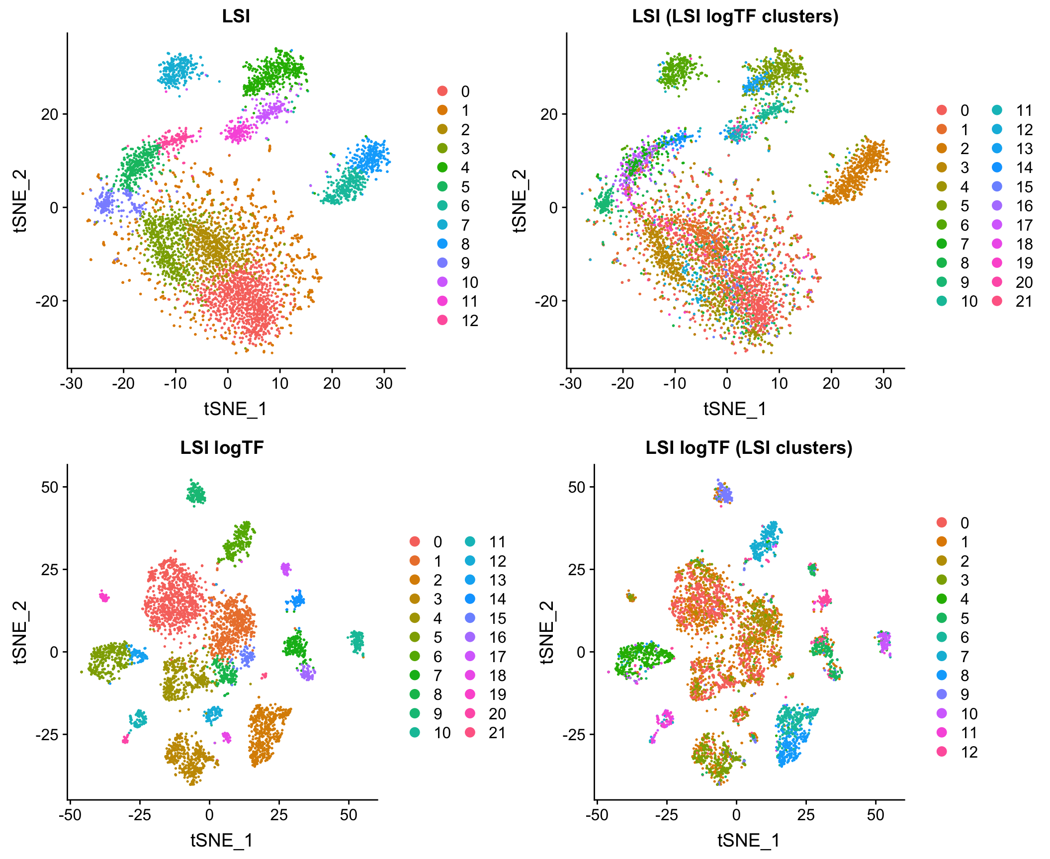
LSI vs. LSI logTF on data from mouse whole brain and PFC

Log scaling the TF matrix tends to improve results markedly. Here is a comparison the original version of LSI (LSI) and the one with a log-scaled TF matrix (LSI logTF) on all whole brain and prefrontal cortex cells from Cusanovich and Hill, et al. Cell 2018 when simply imposing a lower bound on number of cells in which a site is measured as non-zero as a means of feature selection:

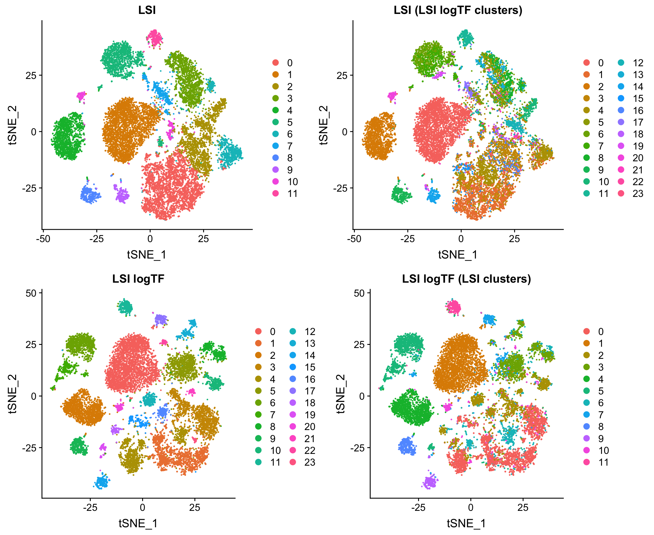
Log scaling makes a big difference here and as you’ll see later, this difference can be even more pronounced on sparser datasets. I’ll refer to this flavor of LSI/LSA as LSI logTF for convenience.

The plot above shows the results of each and then shows what each embedding looks like with cluster assignments swapped between the two techniques to illustrate similarity (or discordance), something I will also do throughout the rest of the post. Note that in each case, I am feeding the reduced dimension space (PCA here) through a standard workflow in Seurat 3 for doing tSNE/UMAP and Louvain clustering. I’ll use this workflow on the initial PCA (or cell by topic matrix for cisTopic) throughout the post to make comparisons between methods as fair as possible.

I admit that evaluating what is “better” or “the same” in each of these comparisons is a bit qualitative. When I make conclusions in this post it is based on the following:

1. Clustering results at identical resolution on PCA (or topic) space having used the same cells and features as input in both methods.
2. Qualitative assessment of large differences in the resulting embedding (in the context of cluster assignments often with high concordance across more than one method). I show tSNE here, but in the R markdown file I also compute UMAP embeddings and these could be plotted instead.

These are not perfect “metrics”, but given that I am largely arguing that LSI/LSA can improved substantially via a simple modification and not trying to make any claims about subtle differences in performance between methods, I think they are sufficient here.

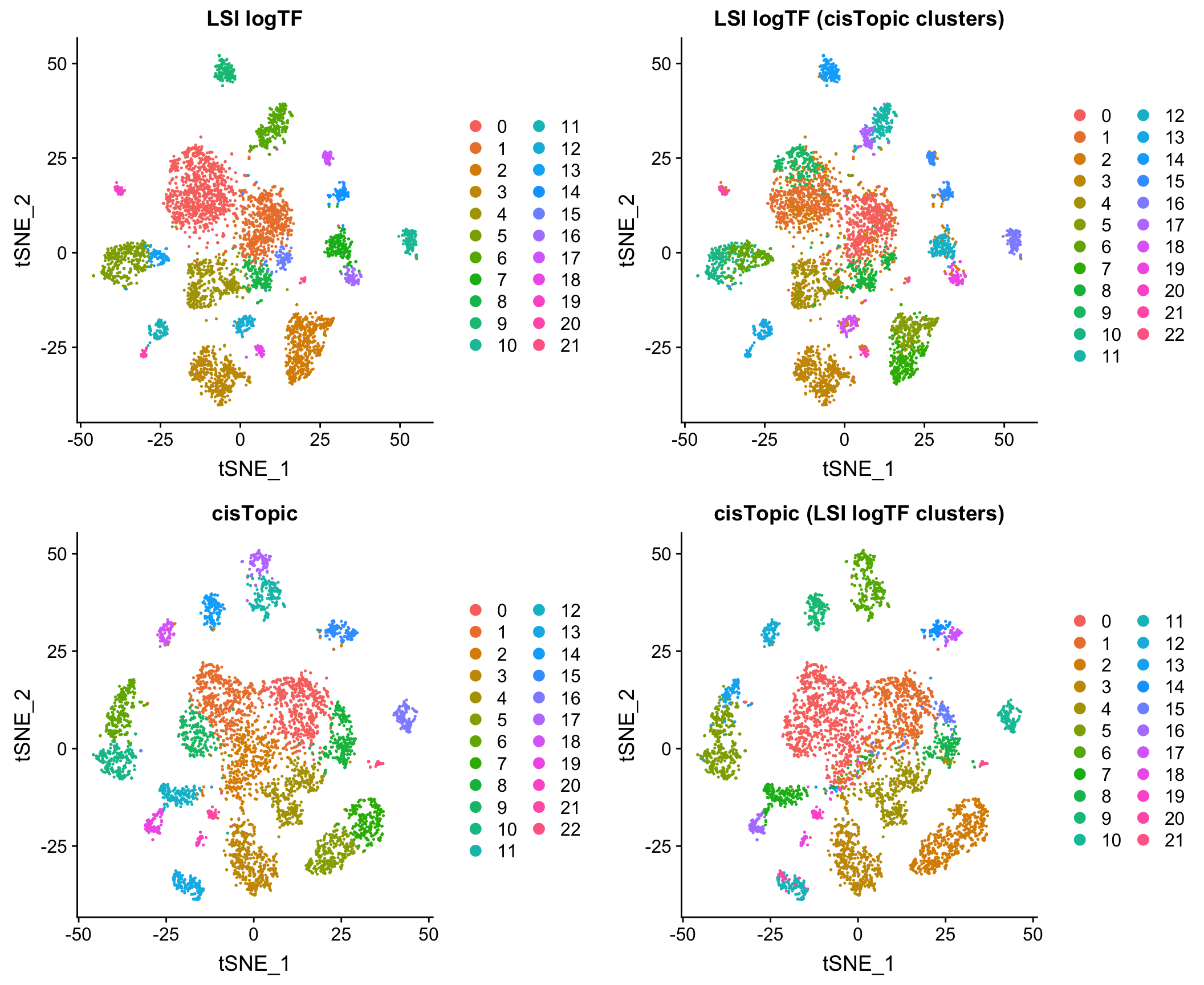
Comparison to cisTopic

Reassuringly, the results look very comparable to those generated by using an LDA-based method, cisTopic (with much shorter runtimes – minutes vs. several hours):

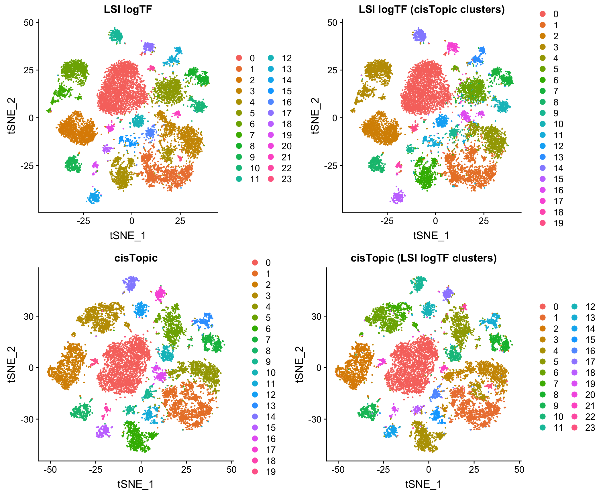
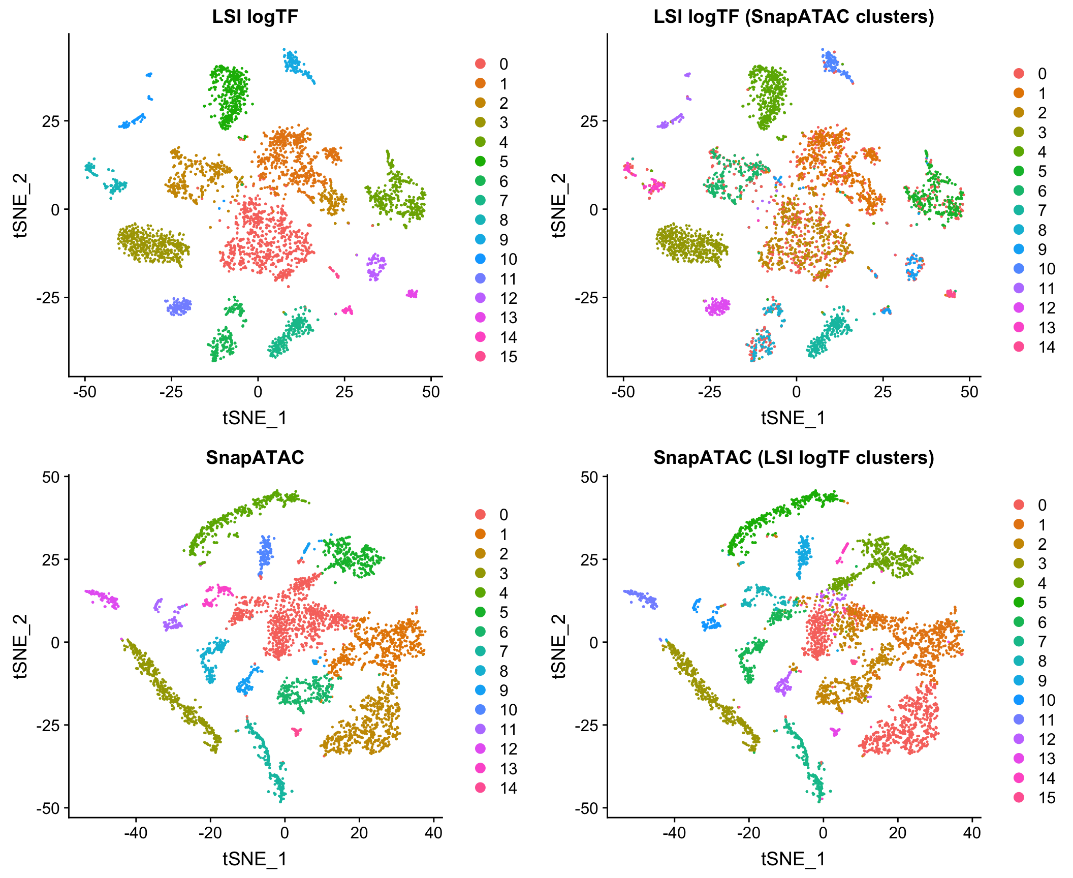
Comparison to Jaccard method

I also compared to the Jaccard-based method in SnapATAC/SnapTools, described in Fang, et al. (bioRxiv 2019). Note that since SnapATAC takes a 5kb window matrix as input rather than peak matrix, I reran LSI logTF on the same window matrix used by SnapATAC to match features and cells used by both methods. This difference doesn’t ultimately matter for this dataset as I’ll show later in the post. I have also chosen to only use the output of SnapATAC up until the PCA stage, using our own common workflow for downstream steps to make a direct comparison.

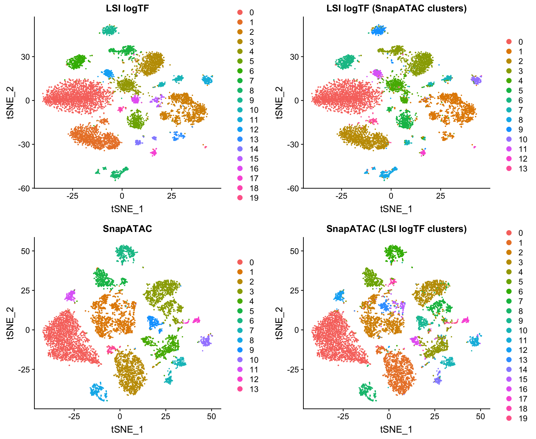
Note that this method uses the binary peak matrix from SnapTools/SnapATAC which ultimately includes a different subset of cells due to QC filtering choices, etc. which seems to account for most of the difference between the use of peaks and windows here with LSI (more on this later). Both of these methods are pretty fast on datasets of this size in my hands.

Comparison to k-mer method

In part, I chose this particular subset of our published data as one of the examples for this post because Lareau, Duarte and Chew, et al. recently published, as part of their supplemental materials, results of applying a 7-mer deviation approach to this same subset of our data. Here is a screenshot of Supplemental Figure 4 panel F from the paper for reference:

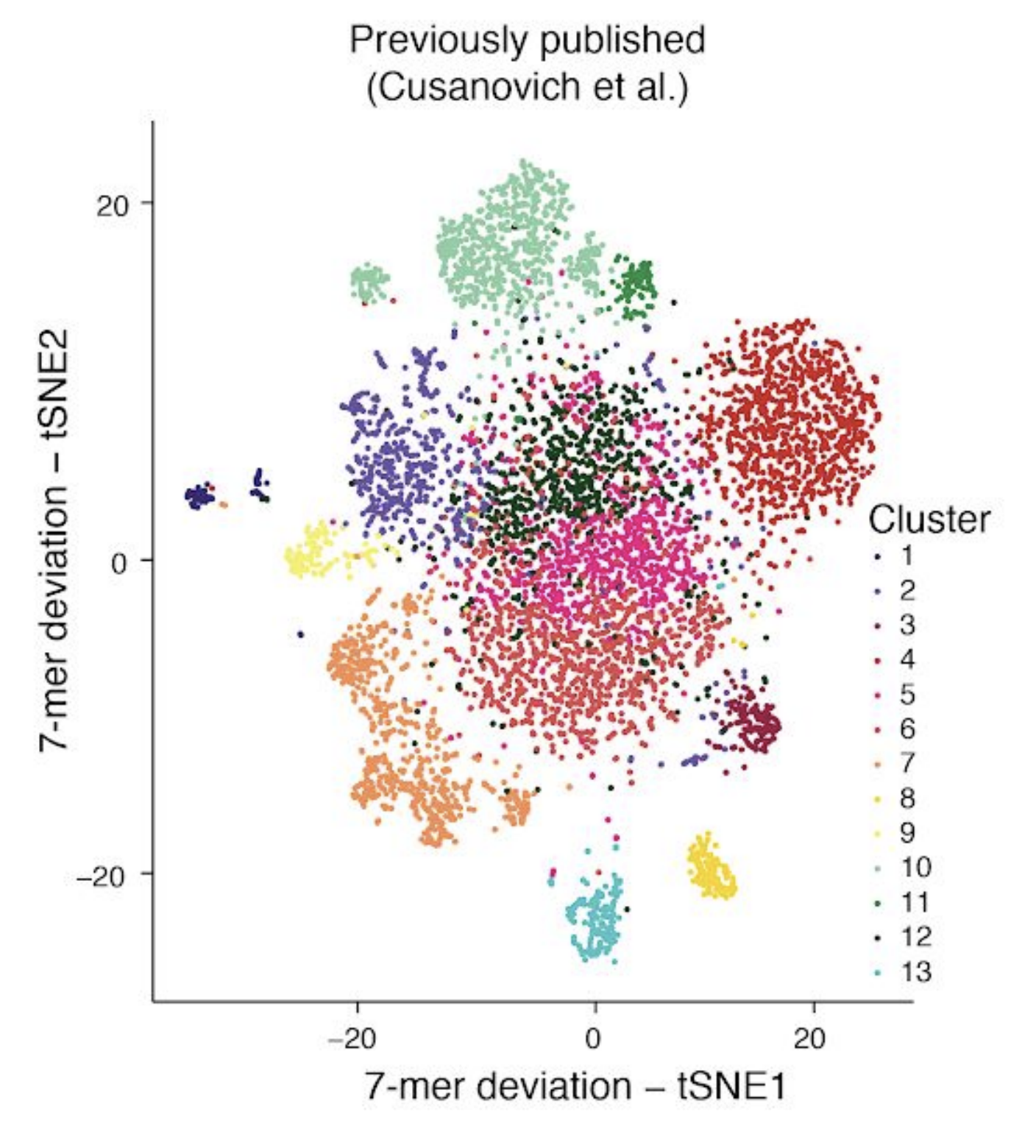
Based on the results above, and independent results from González-Blas, Minnoye, et al. (Nature Methods 2019) and Fang, et al. (bioRxiv 2019) on simulated datasets, I think it is fairly well-established that commonly used approaches that use metafeatures like k-mers don’t tend to perform as well as other alternatives in most contexts. Therefore, I’ve chosen not to compare to these particular methods throughput the rest of this post.

10X adult mouse brain dataset

To show that the above observations also hold true for another dataset (we have anecdotally seen it across many), I downloaded and processed a sample of approximately 5000 nuclei from adult mouse cortex provided by 10x genomics.

Each section follows all the same conventions as the above in terms of input to each tool and plots.

LSI vs. LSI logTF

Comparison to cisTopic

Comparison to Jaccard method

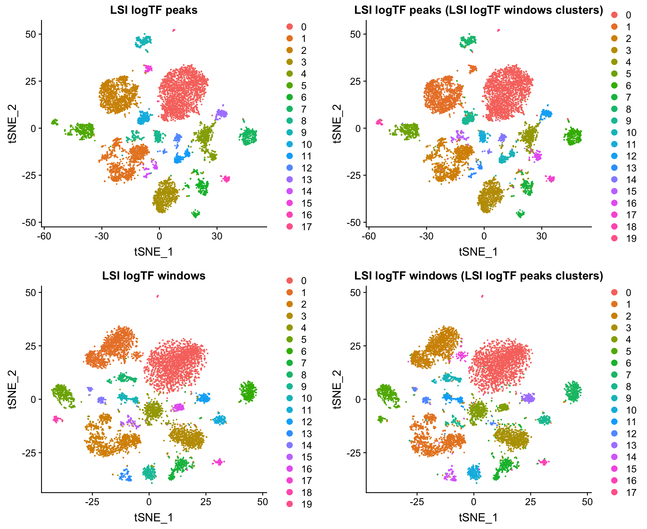
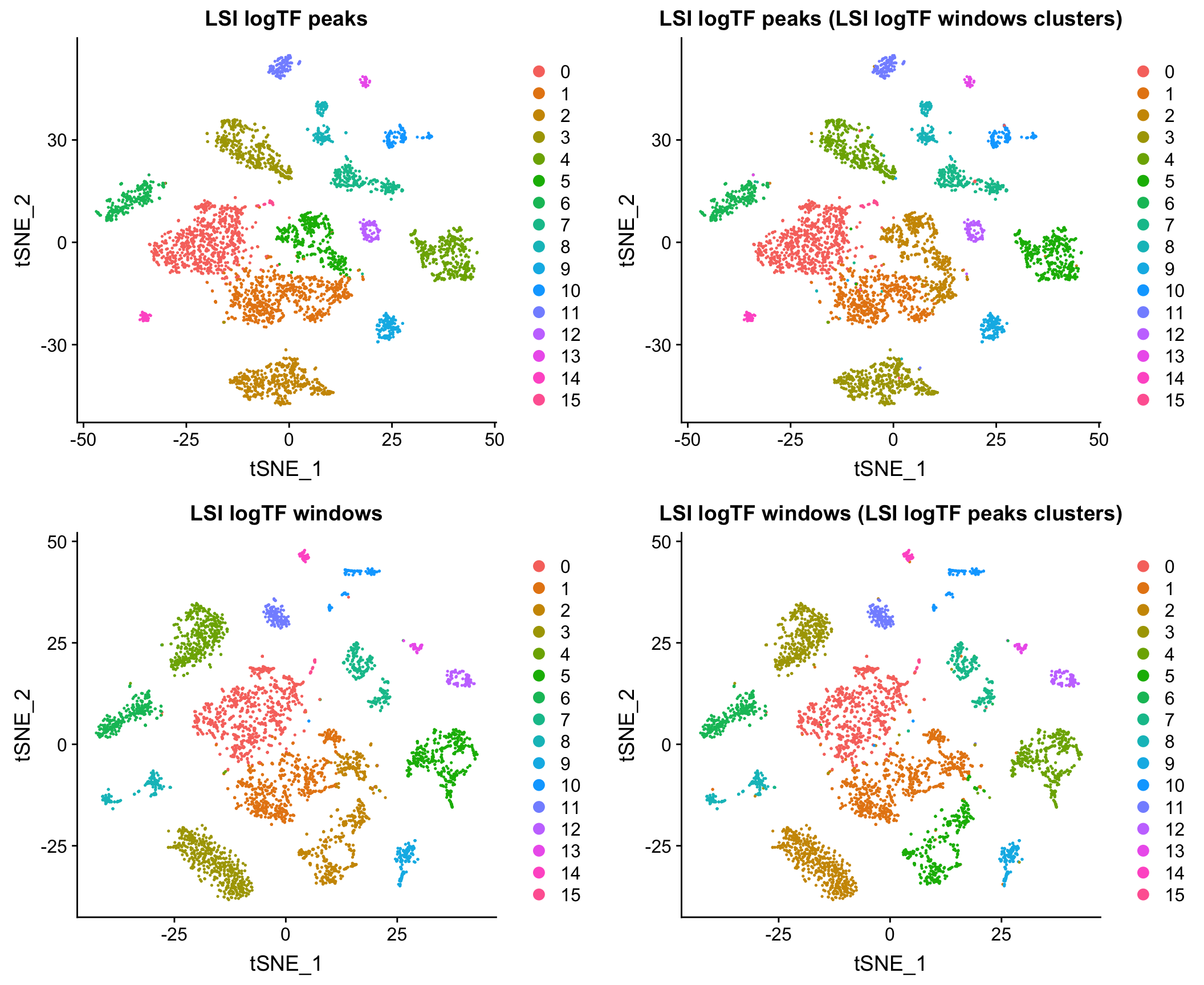
Windows vs. peaks as features

Our lab has historically used peaks as features in most cases (although we have applied LSI to 5kb windows regularly for preliminary clustering steps in all our scATAC-seq publications). Regardless of the choice of dimensionality reduction features, peak by cell matrices (and peak calls more generally) are inevitably quite useful as many analyses are centered around peaks (differential accessibility, motif enrichments, etc.).

However, one thing that scATAC-seq currently lacks relative to scRNA-seq is a common feature set across datasets. If all groups were to report matrices of counts in 5kb intervals (or some agreed-upon length), any two datasets could easily be combined without reprocessing. Peak matrices are inherently sample-specific which means that comparing two datasets would always require having access to BAM files (or something similar) in order to regenerate matrices across common sets of features.

Here I show that at least for the two datasets mentioned above, when matching the cells used as input to the analysis, results using peaks and windows are pretty comparable. More comprehensive assessment would be required to say if either is a better choice in other contexts.

Mouse whole brain and PFC

10X adult mouse brain dataset

Downsampled data

Several papers have examined the impact of decreased complexity on dimensionality reduction results. When starting with a window matrix, if we want to assess the impact of overall complexity on dimensionality reduction, we can just choose a subset of non-zero window-cell entries to zero out at random as an approximate method of downsampling. This task is simplified by the use of windows, since peak calls themselves would be subject to change with decreased depth.

It is worth noting that this by no means captures the real world variation in data quality for scATAC-seq data. Signal to noise ratio (e.g. as measured by FRiP, promoter enrichment, etc.) is also very important and would not be captured by this simple test. Datasets can look very different even at the same overall complexity due to a number of other factors that may differentially impact different methods.

In the interest of time, I chose only to focus on LSI logTF and SnapATAC on the 10x genomics adult mouse brain dataset, but the R markdown file mentioned at the start of the post has all the code one would need to try this out on other datasets. In this case, 20% of the original depth corresponds to only 1-3K unique fragments per cell depending on how you count (quite sparse).

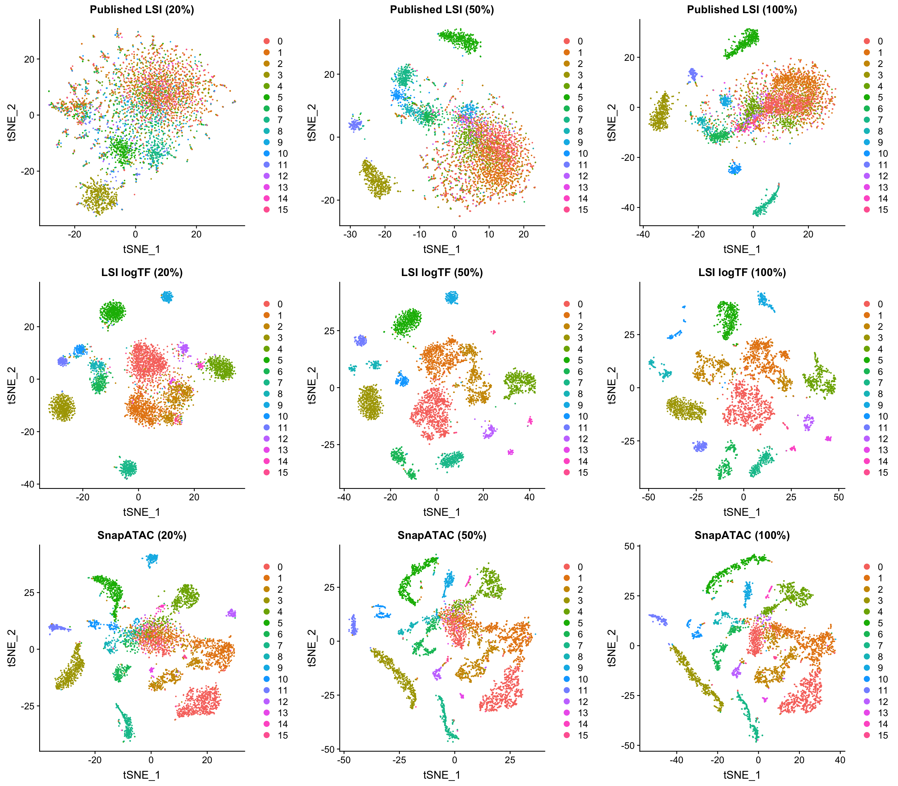
All plots are colored by the original LSI logTF cluster assignments using windows as features. Both SnapATAC and our logTF version of LSI seem to perform quite well at reduced depth. While the plots above look very consistent, there is a slight decrease in the number of clusters called by Seurat for all approaches with downsampling using a consistent resolution parameter (although using a higher resolution paramter would probably enable similar groupings, which is great).

When examining clustering results on each dataset/method independently, LSI logTF has 16, 16, and 11 clusters called at this resolution with decreasing depth (8, 7, and 4 without log scaling). For SnapATAC the number of clusters called has 15, 15, and 13. Therefore, it seems like at least the last downsampling has some deterimental effect in this case for all techniques although I can’t rule out the possibility that choosing a slightly different site-level filtering strategy might make a difference here or that the use of cluster counts here is not slightly misleading in some way (vs. some other more quantitative metric).

At least at this first level of clustering, they seem to perform fairly equitably. It’s possible that one of the two might perform better in an iterative context or other contexts in which there are less obvious differences between cells. In poking around so far, I haven’t found a case where one clearly outperforms the other, but I plan to continue to compare the two on other datasets we’re working with and would be very interested if someone does find good examples.

Conclusions

There are many possible ways in which to reduce the dimensionality of scATAC-seq data and hopefully this serves as a useful review and test of several different methods. I have also shown that even within one class of method (LSI/LSA) simple differences in normalization procedures can make a big difference. Future papers should be careful to document the exact method used (e.g. the equations used for the TF and IDF terms, rather than just stating that LSI/LSA was used). My own personal opinion is that our slightly modified version of LSI/LSA, the Jaccard index based method in SnapATAC, and cisTopic all seem to work quite well even on very sparse datasets. LSI/LSI and SnapATAC have the advantage of being much faster, with cisTopic taking many hours to run on even modestly sized datasets (as also noted in Fang, et al. (bioRxiv 2019)). However, as mentioned above, LDA/PLSI/PLSA have the added benefit of better interpretability given they are probabilistic and cisTopic as a package also has many other nice features independent of dimensionality reduction. While others should explore for themselves to assess performance of these methods in different contexts, my experience so far has been very encouraging. I cannot rule out that there exist other methods not explored here or in other relevant publications that might perform comparably.

Furthermore, the potential for using windows as features could simplify the establishment of common feature sets for scATAC-seq data within the same reference genome. However, I still need to do more exploration in this area.

I would be interested in hearing thoughts from others on this, but it seems like reporting some combination of the following could be quite useful for future studies using scATAC (or other similar measurements):

• BAM files with cell IDs already at the start of the read name or following the typical BAM tag conventions.
• Something resembling the 10x genomics’ fragments file, which represents a more compact representation of relevant data from BAM files.
• A 5kb window matrix as it could then easily be compressed to coarser window sizes if needed without going back to either of the above files. However, providing the BAM/fragments files above would allow for easy generation of matrices with any of a number of common feature sets as needed (e.g. peaks).

Many of the methods discussed here could, in principle, be applied to data from other single-cell epigenetic technologies, not just scATAC-seq.

Note about SnapTools/SnapATAC

Dimensionality reduction is just a very small portion of what SnapTools and SnapATAC accomplish. During the writing of this blog post I have gotten to explore both and think that they are both very useful tools and would encourage others to check them out. SnapTools allows for uniform processing of datasets from different technologies (and is already compatible with outputs of existing pipelines like cellranger-atac from 10x genomics). SnapATAC leverages *.snap files generated by SnapTools to enable lots of extra utilities like wrappers for peak calling and motif enrichment, producing gene level scores, merging of datasets, extraction of reads for subsets of cells, etc. all from a single file. Overall, I have wanted a tool with some of the features in SnapATAC quite badly for a long time and am very thankful that Rongxin Fang and colleagues have developed these tools and made them broadly available.

Note about this post

I wanted to get some of this information out there as I think it is increasingly relevant and I do not currently have the time to polish it up more to put together a bioRxiv post. If there is sufficient interest (e.g. desire to cite), I would consider taking the time to do so in the future.

References

In addition to the 10x genomics scATAC-seq documentation and scATAC-seq datasets (adult mouse cortex used here), I referenced a number of publications in this post.

1. Boer, Carl G. de, and Aviv Regev. 2018. “BROCKMAN: Deciphering Variance in Epigenomic Regulators by K-Mer Factorization.” BMC Bioinformatics 19 (1): 253.
2. Bravo González-Blas, Carmen, Liesbeth Minnoye, Dafni Papasokrati, Sara Aibar, Gert Hulselmans, Valerie Christiaens, Kristofer Davie, Jasper Wouters, and Stein Aerts. 2019. “cisTopic: Cis-Regulatory Topic Modeling on Single-Cell ATAC-Seq Data.” Nature Methods 16 (5): 397–400.
3. Chen, Xi, Ricardo J. Miragaia, Kedar Nath Natarajan, and Sarah A. Teichmann. 2018. “A Rapid and Robust Method for Single Cell Chromatin Accessibility Profiling.” Nature Communications 9 (1): 5345.
4. Cusanovich, Darren A., Riza Daza, Andrew Adey, Hannah A. Pliner, Lena Christiansen, Kevin L. Gunderson, Frank J. Steemers, Cole Trapnell, and Jay Shendure. 2015. “Multiplex Single Cell Profiling of Chromatin Accessibility by Combinatorial Cellular Indexing.” Science 348 (6237): 910–14.
5. Cusanovich, Darren A., Andrew J. Hill, Delasa Aghamirzaie, Riza M. Daza, Hannah A. Pliner, Joel B. Berletch, Galina N. Filippova, et al. 2018. “A Single-Cell Atlas of In Vivo Mammalian Chromatin Accessibility.” Cell 174 (5): 1309–24.e18.
6. Cusanovich, Darren A., James P. Reddington, David A. Garfield, Riza M. Daza, Delasa Aghamirzaie, Raquel Marco-Ferreres, Hannah A. Pliner, et al. 2018. “The Cis-Regulatory Dynamics of Embryonic Development at Single-Cell Resolution.” Nature 555 (7697): 538–42.
7. Fang, Rongxin, Sebastian Preissl, Xiaomeng Hou, Jacinta Lucero, Xinxin Wang, Amir Motamedi, Andrew K. Shiau, et al. 2019. “Fast and Accurate Clustering of Single Cell Epigenomes Reveals Cis-Regulatory Elements in Rare Cell Types.” bioRxiv. https://doi.org/10.1101/615179.
8. Graybuck, Lucas T., Adriana Sedeño-Cortés, Thuc Nghi Nguyen, Miranda Walker, Eric Szelenyi, Garreck Lenz, La ’akea Sieverts, et al. 2019. “Prospective, Brain-Wide Labeling of Neuronal Subclasses with Enhancer-Driven AAVs.” bioRxiv. https://doi.org/10.1101/525014.
9. Ji, Zhicheng, Weiqiang Zhou, and Hongkai Ji. 2017. “Single-Cell Regulome Data Analysis by SCRAT.” Bioinformatics 33 (18): 2930–32.
10. Lake, Blue B., Song Chen, Brandon C. Sos, Jean Fan, Gwendolyn E. Kaeser, Yun C. Yung, Thu E. Duong, et al. 2018. “Integrative Single-Cell Analysis of Transcriptional and Epigenetic States in the Human Adult Brain.” Nature Biotechnology 36 (1): 70–80.
11. Lareau, Caleb A., Fabiana M. Duarte, Jennifer G. Chew, Vinay K. Kartha, Zach D. Burkett, Andrew S. Kohlway, Dmitry Pokholok, et al. 2019. “Droplet-Based Combinatorial Indexing for Massive Scale Single-Cell Epigenomics.” bioRxiv. https://doi.org/10.1101/612713.
12. Lopez, Romain, Jeffrey Regier, Michael B. Cole, Michael I. Jordan, and Nir Yosef. 2018. “Deep Generative Modeling for Single-Cell Transcriptomics.” Nature Methods 15 (12): 1053–58.
13. Preissl, Sebastian, Rongxin Fang, Hui Huang, Yuan Zhao, Ramya Raviram, David U. Gorkin, Yanxiao Zhang, et al. 2018. “Single-Nucleus Analysis of Accessible Chromatin in Developing Mouse Forebrain Reveals Cell-Type-Specific Transcriptional Regulation.” Nature Neuroscience 21 (3): 432–39.
14. Satpathy, Ansuman T., Jeffrey M. Granja, Kathryn E. Yost, Yanyan Qi, Francesca Meschi, Geoffrey P. McDermott, Brett N. Olsen, et al. 2019. “Massively Parallel Single-Cell Chromatin Landscapes of Human Immune Cell Development and Intratumoral T Cell Exhaustion.” bioRxiv. https://doi.org/10.1101/610550.
15. Schep, Alicia N., Beijing Wu, Jason D. Buenrostro, and William J. Greenleaf. 2017. “chromVAR: Inferring Transcription-Factor-Associated Accessibility from Single-Cell Epigenomic Data.” Nature Methods 14 (10): 975–78.